Lecture 1

6/2/2019

-Correlation is about two variables being associated, but there is no evidence of causality. 

-Causality however requires multiple factors: covariance (variables have an association), directionality(cause precedes effect (in time)) and internal validity(eliminate alternative explanations).

- Correlations can be displayed in scatterplots that show:

       - Direction: positive or negative

       - Strength: density of the points

       - Shape: linear/nonlinear and homogeneous (one cluster) / heterogeneous (multiple clusters).                 

       - Outliers

-Covariance (s_xy): to measure the degree to which two variables vary together.

            Formula:  s_xy = Σ(x_i-x)(y_i-y) / N-1

It provides us with information on the strength and direction of the association. The disadvantage is that the covariance is dependent on the unit of measurement of the variables.

-Pearson r is a standardized measure that describes the linear relationship between two quantitative variables, and always lies between -1 and +1.

            Formulas:        r = s_xy / s_xs_y            Alternative:     r = Σz_xz_y / N-1 

- Remember that a z-score is a standardized score that displays how many standard deviations a certain score is away from the mean.

Alternative correlational techniques:

- The Pearson r is the correlation coefficient that is most commonly used. There are alternatives:

quantitative + quantitative      --> Pearson r

ordinal + ordinal                     --> Spearman’s rho (r_s)

dichotomous(only two possible values)+ quantitative --> point-biserial correlation (r_pb)

dichotomous + dichotomous  --> phi coefficient (ϕ)

-Spearman’s rho  (r_s) describes relationship between two ordinal variables/ranked scores.

            Formulas: x_rank = N + 1 / 2        s_rank = √ (N(N+1) / 2)                             

           r_s = r on ranked data

Spearman’s rho is also an alternative to Pearson r in case of outliers and/or weak non-linearity.

-Point-biserial correlation describes relationship between quantitative and dichotomous variables. We use the Pearson correlation formula to calculate r_pb:    r_pb = r

The sign of the correlation (+/-) depends on the way 0 and 1 are assigned to groups.   

            Relationship r_pb and t_independent:     r_pb = Square root of t² / t² + df         

-Phi-coefficient (ϕ) describes relationship between two dichotomous variables:     ϕ = r

There is also a specific formula to calculate ϕ when you make a 2✕2 contingency table:  

       ϕ = √ (AD - BC / (A+B)(C+D)(A+C)(B+D) )       

Relationship ϕ and χ²:           ϕ = √(χ² / N)               χ²= ϕ² ✕ N

- Testing the significance of r, r_s, r_pb or ϕ:                t = r √ N-2 / √1-r²        with df = N - 2.

- Testing the difference between two independent r’s:     z = r'₁ - r'₂ / √ 1/N₁-3 + 1/N₂-3    

Important is to transform r to r’ first, according to Fisher's table.

- Statistical significance depends on N, r and α; so weak correlations in large samples can become significant and strong correlations in small samples might not be significant. So, testing only for significance is too limited.

- Measures of effect size: r_effect, r² (COD, VAF), Cohen’s d or Hedges’s g

- Correlation r is already an effect size; r_effect

- The advantage of r²‘s (Coefficient Of Determination; COD, or Proportion of Variance Accounted For; VAF) is that we can compare them. But using r² also has drawbacks.

- Cohen’s d and Hedges’s g are suitable for comparing the means of two groups (r_pb).

            Cohen’s d: |μ₁ - μ₂ | / σ

            Hedges’s g: |x₁ - x₂| / s_p            

The formulas were especially designed to leave out the size of N (~> comparison to t)

- Rules of thumb: 

                d/g           r              r²           r_pb             r²_pb

Small       0.20         0.10         0.01        0.10          0.01

Medium    0.50         0.30         0.09        0.24          0.06

Large       0.80         0.50         0.25        0.37          0.14

Lecture 2

13/2/2019

Simple linear regression:

- Correlations describe linear associations between two (interval) variables.

Regression enables you to estimate one interval variable from one or more others.

- In regression there is a clear distinction between the predictor variable (X) and the response/criterion variable (Y).

- 1 predictor variable --> simple linear regression

2 predictor variables --> multiple linear regression

- (Unstandardized) regression equation:        (^ indicates an estimation)

            b₀= intercept/constant: predicted value of y when x = 0

            b₁= slope: size of the difference in y^{^} when x increases by 1 unit            

- Error/residual (e_i) = the difference between observed (y_i) and predicted value (y^{^}_i)

Best fit of the data when Σe_i is minimized.

-b₀ = y^bar - b₁x^bar

b₁= s_xy / s²_x                 = r * s_y / s_x

-Interpolation is making a prediction within the range of X and Y

Extrapolation is making a prediction outside the range of X and Y

- Problem; when the unit of measurement changes, regression equations change as well. So we use standardized regression equations:        z^bar_y = rz_x

Accuracy of prediction:

- How good is the model: Our data consist of explained data and some error/unexplained data. Best fit of the data when Σe_i²  is minimized

- Total variance:        SS_total / df_total          Σ(y^hat-yb^ar)² / N-1  (N-1 are the degrees of freedom of y)

Model variance:        SSmodel/ dfmodel         Σ(y^hat-yb^ar)² / p     (p is the number of predictors)

Error variance:         SS_error / df_error          Σ(y-yb^ar)² / N-2     (N-2 are the degrees of freedom of e)

- VAF = 1 - (SS_error / SStotal)    -->       SS_y = s²_y* df_total

For simple linear regression also holds:       VAF = r²

Significance testing:

- μ_y= β₀ + β₁x  with variation σ

1_1.--> β₀ is estimated with b₀, β₁is estimated with b₁, σ is estimated with s_e.

- t =  b₁ / SE_b1              SE_b1 = s_e /s_x √N-1                                - 

- Confidence interval for b₁:  b₁± t * SE_b1, where t* is two-tailed critical t value with df=N-2

- If p < 0.05, X is a significant predictor of Y.

- Testing significance of two independent regression weights: (b_1.1means b1 in sample 1)

t = b_1.1 - b_1.2 / s_b1.1-b.1.2     df = n₁+ n₂– 4        s_b1.1-b1.2 = √s²_e.1 / s²_x.1 (N₁ - 1) + s²_e.2/ s²_x.2 (N2 - 1)             

Lecture 3

20/2/2019

- With multiple linear regressions, we have 1 response variable (y) and multiple predictor variables (x₁, x₂, et cetera). When we have more predictor variables, we will be able to estimate the response variable better and deal with less error variance. The multiple predictor variables do have to be related. 

- Regression equation sample:    y^{^} = b₀ + b₁x₁ + b₂x₂    ... + b_px_p          

Regression equation population: μ_y = β₀ + β₁x₁ + β₂x₂      ... + β_px_p

- In multiple linear regression, the regression coefficient indicates the effect of x on y while controlling for the other predictor variables/keeping the other predictor variables constant.

- With two predictors, the relationship can be represented by a regression plane (a 3D scatterplot). The vertical distance from a point (y) to the plane ( is the error e_i).

- Variances (mean squares):

-> Total variance:      MS_y = SSy / df_y            = Σ(y^hat-yb^ar)² / N-1  

Model variance:        MS_yhat = SSyhat/ df_yhatl    = Σ(y^hat-yb^ar)² / p     

Error variance:         MSe = SS_error / df_error      = Σ(y-yb^ar)² / N-2       

- VAF (Proportion Explained Variance): SS_yhat / SS_y          VAF = R²         

- R = the correlation between  and y, the multiple correlation coefficient.

R²= the proportion explained variance / VAF

R²_adj = the estimate of proportion explained variance in the population; 

- Testing the regression model:

1)       H₀: R²= 0                    H_a: R²> 0        

          H₀: β₁= β₂= 0             H_a: at least one β_j ≠ 0             

          H₀: R = 0                     H_aR > 0          (cannot be negative)

2) ANOVA F-test for regression: F (df_yhat, df_e) = MS_yhat / MS_e    with df_yhat = p   and df_e= N – p – 1

Notes: in simple regression F is equal to t², but not in multiple regression. 

- F is a test statistic, like t or z. It looks at the ratio between unexplained and explained variance; the larger the test statistic, the smaller the p-value. F is always a positive value, since variances cannot be lower than 0.

3) Look up the F-value in the table to get a p-value.

4) Draw the statistical and substantive conclusion: If p < α, H₀ is rejected and the results of the regression indicate that the two predictors collectively explain the VAF.

- Adding up the VAF of two predictors through simple regression analysis gives an other value than the VAF of these predictors through multiple regression. This is because one predictor explains a part of the variance of the response variable that the other predictor does too

- Semipartial correlation:

r_0(1.2)= the correlation between y and part of x₁that is independent of x₂, so in other words the correlation between y and partly x₁after correcting for the overlapping part with x₂.

Semi-partial correlations in SPSS --> “Part correlations”

r_0(1.2) = √ B / A+B+C+D

-Partial correlation:

r_01.2= the correlation between y and part of x₁that are both independent of x₂:

r_01.2 = √ B / A+B

- Testing the Multiple Regression Coefficient:

H₀: β_j= 0         H_a: β_j≠ 0 / H_a: β_j< 0

t = b_j / SE_bj     with df_e= N – p – 1                

--> Look up p-value in t-table and draw conclusions about the significance of predicting y for each of the predictor variables.

Confidence Interval for b_j:     b_j ± t × SE_bj

- Predict Y from X₁and X₂

Simple regression:     Response variable (Y) and predictor (X; one of both)

Multiple regression:    Response variable (Y) and predictors (X₁ and X₂)

-Spurious relations can be the result of a relation between X₁and X₂if we’ve only dealt with the relation between X₁and Y. Controlling for X₂should eliminate this spurious effect. We do this by using a multiple regression analysis.

Lecture 4

28/2/2019

- Assumptions for regression analysis:           

     --> Linearity: There is a linear relation between the predictor variables and the              response variable.

   --> Homoscedasticity: The variance of the residuals is equal for each predicted value. In a scatterplot showing homoscedasticity, the point are randomly distributed around a horizontal line. For heteroscedasticity, the point cloud varies in width; isn’t concentrated around a horizontal line.

   --> Normality of the residuals: The residuals are normally distributed for every predicted value.

- When any of these assumptions are violated, the variable needs to be transformed. It this isn’t effective ~> restraint interpreting tests.

- With multicollinearity, two or more predictor variables are strongly intercorrelated (with an r higher than 0.70 or 0.80). Consequently, regression coefficients become unstable and standard errors increase. It is more difficult to find significant effects.

- Check:          Tolerance: 1 – R²(as high as possible)

                       Variance Inflation Factor (VIF): 1 / tolerance (as low as possible)

If the tolerance is much larger than 0.10, and the VIF is much smaller than 10, there is no multicollinearity.

- If multicollinearity does exist, a variable needs to be removed from the regression model or predictors need to be combined into a sum score/scale.

- Test whether there are outliers on your data:

            1) Distance: are the scores on Y much higher/lower than expected (look at the            standardized residuals; higher than |3| are outliers).

            2) Leverage: are there outliers on the predictors? (look at leverage values; 3(p+1) / N --> outlier on predicto

            3) Influence: how much does an observation influence the results? (values smaller than 1 on Cook’s Distance are not influential).

- Is there no apparent reason for your outliers? Do not remove them! Apparent reason for removing outliers can be that it’s about an impossible score (due to data entry errors) or that it’s about an observation than is very different (e.g. a male in a female sample by accident).

-Selection methods: 

Standard (Enter): All predictors are added simultaneously.

Stepwise: Predictors are added on the basis of their unique VAF

Hierarchical: Predictors are added in an order determined by the researcher.

-Confidence Interval (CI):            μ^ ± t* × SE_μ^

with SE_μ^: s_e= √1/N + (x-x^bar)² / (N-1)s²_x

and t* from t table with df = N – p – 1

-Prediction Interval (PI):   y^ ± t* SE_y^

with SE_y^: s_e= √1 + 1/N + (x-x^bar)² / (N-1)s²_x

and t* from t table with df = N – p – 1 

- The predictor interval is always wider then the confidence interval. Intervals get wider as they get further away from the x^bar.

-Mediation: When a predictor X indirectly affects the response Y.

Moderation: When the strength of the relation between X and Y depends on another variable.

Lecture 5

6/3/2019

- During this lecture, all the topics of the past lectures were reviewed.

New topics:

- During regression analysis, categorical variables can be included using dummy variables, which are dichotomous variables with 0 and 1. Advantages: look at differences between groups (means) and look for possible interaction.

- Testing interaction uses the same testing procedure as with testing two independent regression coefficients (see lecture 2).

Lecture 6

13/3/2019

- The problem of analysing multiple t-test to draw one conclusion is that the probability of Type I error increases (more about this effect will be explained in next week’s lecture), so we use Analysis Of Variance (ANOVA).

- ANOVA hypotheses:          H₀: μ₁= μ₂= ... μ_I

                                                                    H_α: NOT μ₁= μ₂= ... μ_I            

So what the ANOVA test does, is determining whether all the population means are equal or if there is a difference between at least two of them (= omnibus test).

- 1 categorical X variable --> One-way ANOVA

2 or more categorical X variables --> Factorial (or two-way) ANOVA

- The F-test compares differences between groups (explained) with differences within groups (unexplained).

- One-way ANOVA model:

            Data (total) = Fit (between) + Residual (within)

            y_ij = μ_i + ε_ij

            y_ij = μ + α_i  + ε_ij

In which i = condition, j = participant, α_i  = effect parameter (= the effect of a certain condition compared to the grand mean); (μ_i – μ) 

- Parameters in One-way ANOVA:

            y_ij = μ_i + ε_ij

            y_ij = μ + α_i + ε_ij

- μ is estimated with y^bar, μ_i is estimated with y^bar_i , α_i  is estimated with α^ = y^bar_i - y^bar  and σ is estimated with s_p.

- Assumptions of the ANOVA model:           

            1. Homogeneity of variances 

The variance of residuals is same in all populations: The rule of thumb is the largest sd / smallest sd < 2, or you can check the significance of Levene’s test.

            2. Normality of the residuals

The residuals are normally distributed within each group (mean 0 and standard deviation σ): Look at histogram or P-P / Q-Q-plot of the residuals.

            3. Independence

The residuals are independent: This should be guaranteed by the design of the study.

If the assumptions of homogeneity and/or normality are violated, you have to check the data set for error and outliers, or transform the Y variable or use a non-parametric test (Kruskal Wallis).

- Kruskal Wallis test hypotheses:

            H₀: MR₁= MR₂= ... MR_I

                   H_α: NOT MR₁= MR₂= ... MR_I

- ANOVA table:

            Source           Sum of Squares       df        Mean Square                      F

            Groups           SS_G                             df_G       SS_G / df_G                     MS_G / MS_E

            Error               SS_E                             df_E       SS_E / df_E

            Total                SS_T                             df_T       SS_T/ df_T

The F-test looks at the ratio between explained (groups) and unexplained (error) variance:

F = MS_G/ MS_Ewith df_Gand df_E.

- SS_T= Σ (y_ij -  )²                 (difference between individual scores and grand mean) 

            > with df: N – 1

SS_G= Σ n_i(y_ij -  )²= Σ n_i α^_i    (differences between group means and grand mean)

           > with df: I – 1     (I is the number of conditions/groups)

SS_E= Σ (y_ij - _i)²                       (difference between individual scores and group means)

                  > with df: N – 1

- So: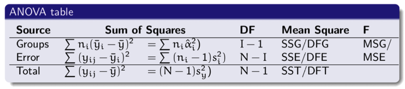 

(Source: Lecture slides week 6, slide 17, Hemmo Smit, Leiden University)

- Note that SS_T= SS_G+ SS_E, df_T= df_G+ df_E; but MS_T≠ MS_G+ MS_E

- When p < α, the F test has showed that the groups are significantly different.

- Measures of effect size:     

VAF in ANOVA is denoted by η² instead of R²                          η²= SS_G/ SS_T                   

- η² is based on sample statistics, but consequently overestimates the population value. Therefore we use ω^²:                                                                        ω^²= SS_G– (df_G* MS_E) / SS_T+ MS_E

This value is always lower than η².

- Conclusion: estimated that in our population the 'between groups-factors  explain ω^² (percentage value) of the variance in Y.

- Rules of thumb for the effect size:       small: .01        medium: .06    large: .14

Lecture 7

20/3/2019

- Why we cannot use results of multiple t-test to compare more than two group means:

Type I error is rejecting H₀when it was in fact correct. When we perform multiple t-tests, we get an increased type I error. 

-Familywise error: α_fam = 1 – (1-α)^c                    in which c = the number of comparisons.

- Solution: ANOVA F test; this compares all means simultaneously, so there is no increased type I error.

- ANOVA tests give us indications whether at least two group means differ significantly from each other. However, we don’t know which ones:

- To know which group means are significantly different from one another we can make:

            - A priori comparisons; contrasts (planned comparisons)

                       Contrasts are specified before the data is collected.

            - A posteriori comparisons; post-hoc comparisons

                       Additional test done after significant F-value is found to determine which                                     means are significantly different.

- Examples for a priori hypotheses:

            H₀: (μ₁ +μ₂) / 2 = μ₃     H_α: (μ₁+μ₂) / 2 > μ₃        (one-sided)

                  H₀: μ₁= μ₂                  H_α: μ₁≠ μ₂                   (two-sided)

- To determine a priori contrasts we formulate linear contrasts (ψ): combination of population means. The goal is to compare (groups of) means.

            ψ = α₁μ₁+ α₂μ₂+ ... α_kμ_k                         (α_i are contrast coefficients)

- These contrast coefficients are weights. Groups with positive coefficients are compared with groups with negative coefficients. Contrast coefficients can be multiplied, as long as it’s with the same value, so that: Σα_i = 0.

- Contrast can or cannot be orthogonal; independent. Criteria for being orthogonal:Σα_i= 0, Σb_i= 0, Σα_ib_i= 0, and the number of comparisons: DFG = I – 1.

- t-test for contrasts:t = c / SE_c       = Σα₁x^bar_i / s_p √Σα²_i/ n_i         with df = DFE = N – 1

c = sample contrast

SE_c= standard error of sample contrast

s_p= pooled standard deviation (equal to √MSE)

- For testing a significant ANOVA F-test is not required.

- Contrasts in SPSS: Analyze --> Compare Means --> One-way ANOVA --> Contrasts

Specify α_is one by one (Coefficients --> Add). With “Next” it is possible to specify multiple contrasts. α_is should always add up to zero (the Coefficient Total).

- Conclusion: when p < α, y did not significantly differ between group 1 and group 2. Or: when p < α, y significantly differed for group 1 compared to the other groups.

- Other contrasts in SPSS:    simple (first): each group is compared with the first group.

                                          simple (last): each group is compared with the last group.

                                          repeated: each group is compared with the next group.

                                          polynomial: look at trend in data (linear, cubic, et cetera).

-Bonferroni Correction: corrects for when testing multiple contrast leads to an increased probability of Type I error.

            α’ = α/c           (c = number of comparisons)

Compare the p value with this corrected α. Using the Bonferroni Correction does decrease the power.

-Post-hoc tests are additional test (pairwise comparisons) that are done when the F-test is significant, but no specific hypotheses were formulated.

- There are multiple different tests:

--> Bonferroni corrections are done for a priori tests (a more conservative method; so we loose more power):          α is adjusted by dividing it by the number of comparisons.

            m (m-1)  / 2     (m = the number of conditions)

--> Tukey corrections are done for post hoc tests. It essentially does the same thing as Bonferroni.

In SPSS: One Way ANOVA --> Contrasts --> Bonferroni / Tukey

- t** indicates a corrected t variable.

Lecture 8

27/3/2019

- Factorial designs include multiple independent variables. 

- The outcome indicates the main effects; overall effect of each factor separately, and the interaction effects; the effect of one factor dependent upon the level of the other factor.

- Advantages of factorial designs: 

1. Improved generalizability; by controlling for a hidden variable

2. More efficient research; better than doing two separate experiments with same number of participants per condition.

3. Increased power; the second factor in the model leads to a smaller error variance.

4. Interaction; investigates the interaction between two variables.

- One-way model:      y_ij = μ+ α_i + ε_ij             

            where i = condition and j = participant.

- Factorial model:        y_ijk = μ + α_i + β_j + αβ_ij + ε_ijk      

            where i = condition factor A, j = condition factor B and k = participant

μ is estimated with y^bar

μ_ijis estimated with y^bar_ij

α_iis estimated with α^_i = y^bar_i- y^bar

β_jis estimated with β^_j= y^bar_j - y^bar

αβ_ijis estimated with α^β_ij = y^bar_ij – (y^bar+ α^_i+ β^_j)

σ is estimated with s_p

- (Checking) assumptions in factorial ANOVA:

            1) Homogeneity of variances; variances of residuals is the same in all populations:

                       largest sd / smallest sd < 2 or check Levene’s test.

            2) Normality of residuals; residuals are normally distributed within each group 

                       Check with the histogram or P-P/Q-Q plot of the residuals

            3) Independence of residuals

                       Is guaranteed by the design.

- ANOVA table: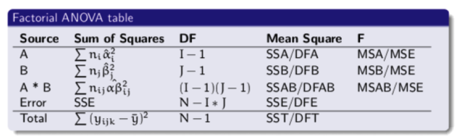 

(Source: Lecture slides week 8, slide 11, Hemmo Smit, Leiden University)

- F-test looks at the ratio between explained effect and unexplained variance:

F = MS_effect/ MSE        with df_effectand df_E

- SS (Corrected Total)           = SS (Corrected Model)         + SS(Error)

            SST                            = SSM                                    + SSE

- Effect size for factorial ANOVA:

            > Total VAF in sample:                      η²= SSM / SST

            > VAF by effect in sample:    η¹= SS_effect/ SST

            η²_partial= SS_effect/ (SS_effect + SSE)

            Rules of thumb:          0.01 = small    0.06 = medium            0.14 = large

            > Estimated VAF by effect in population:      ω^²= SS_effect – (df_effect * MSE) / SST + MSE